Skip to the examples

D3 - Chart.js - Recharts - Teaching gallery

Six chart examples

Six small demos, each showing a different way to turn data into a chart.

Open a demo to see it working, then use Details to read how the chart was made. Ask your tutor if you want the original source code.

Examples

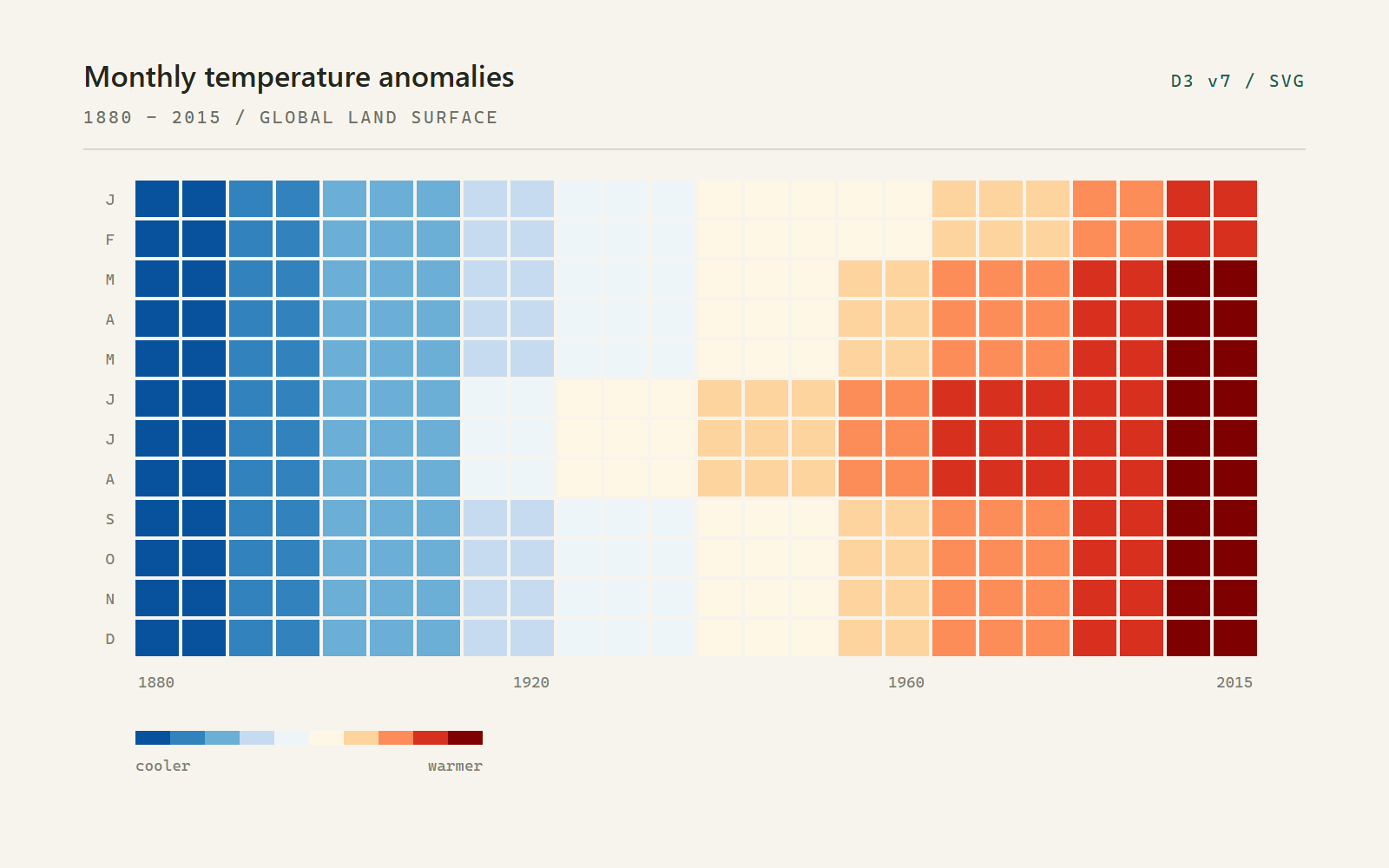
A blue-to-red heatmap grid showing monthly global temperature anomalies from 1880 to 2015.
Preview of the monthly temperature heatmap demo.
01 D3 v7 - SVG

Monthly temperature heatmap

Each square is one month. Year runs along the x-axis, month down the y-axis, and colour shows whether that month was cooler or warmer than the 1951-1980 average.
Open demo
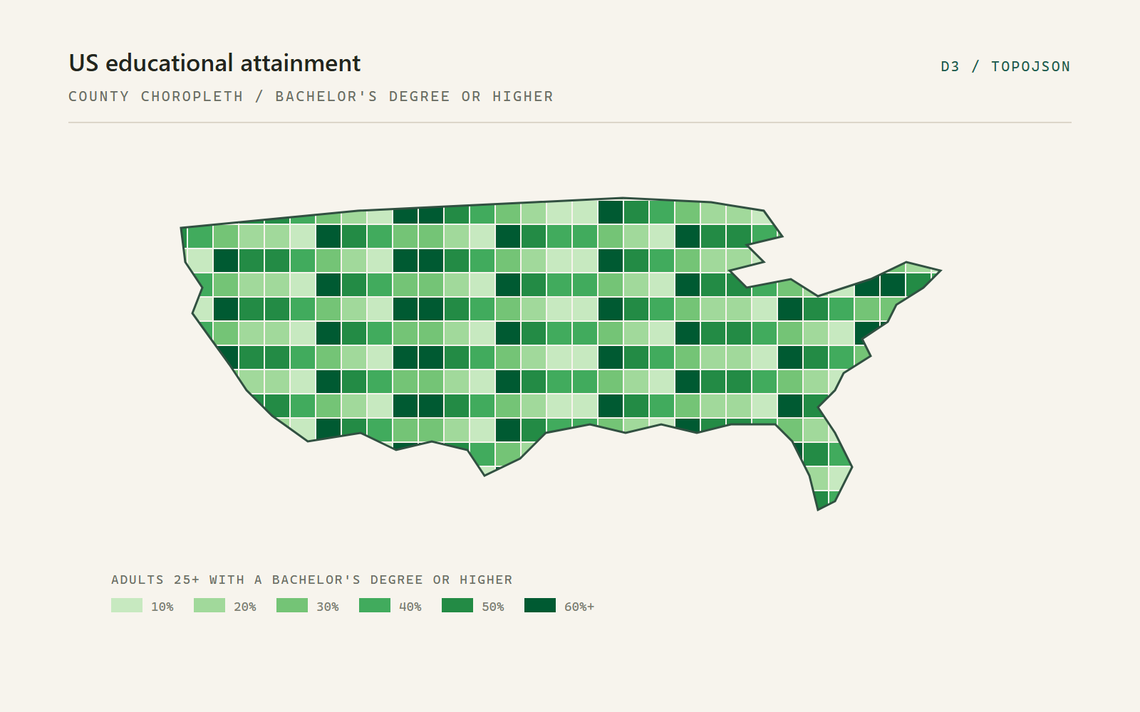
A county-level choropleth map of the United States shaded in bands of green.
Preview of the US education choropleth demo.
02 D3 v7 - TopoJSON

US education choropleth

A map of the United States, county by county. The green shading shows the share of adults aged 25 and over with a bachelor's degree or higher. Hover over a county to see its name and value.
Open demo
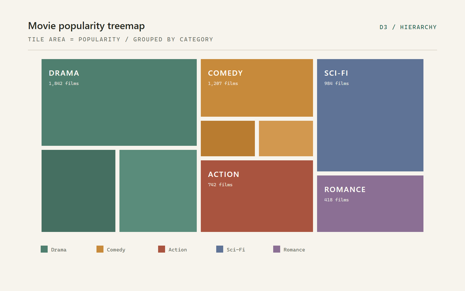
A movie popularity treemap made of nested coloured rectangles grouped by genre.
Preview of the movie popularity treemap demo.
03 D3 v7 - Hierarchy

Movie popularity treemap

Every rectangle is a film. The size shows its popularity and the colour shows its genre, so the biggest genres take up the most space.
Open demo
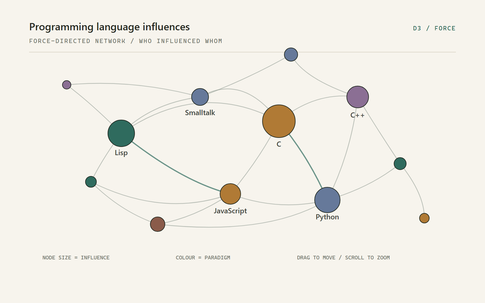
A force-directed network of programming languages shown as coloured circles joined by curved links.
Preview of the programming language influence graph demo.
04 D3 v7 - Force

Programming language influences

Each circle is a programming language. Bigger circles have influenced more languages, colour shows the paradigm, and the lines show which language influenced which.
Open demo
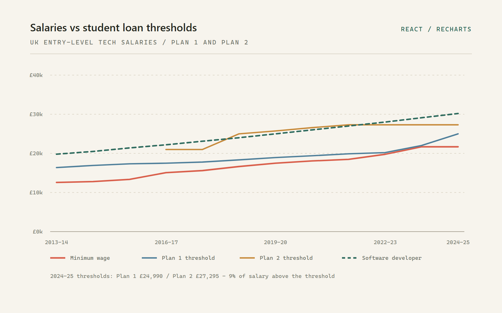
A line chart comparing UK minimum wage and career salaries with student loan repayment thresholds.
Preview of the salaries versus student loan thresholds demo.
05 React - Recharts

Salaries vs student loan thresholds

Compare entry-level tech salaries with Plan 1 and Plan 2 student loan repayment thresholds, from 2013-14 to 2024-25. Choose a career to update the chart.
Open demo
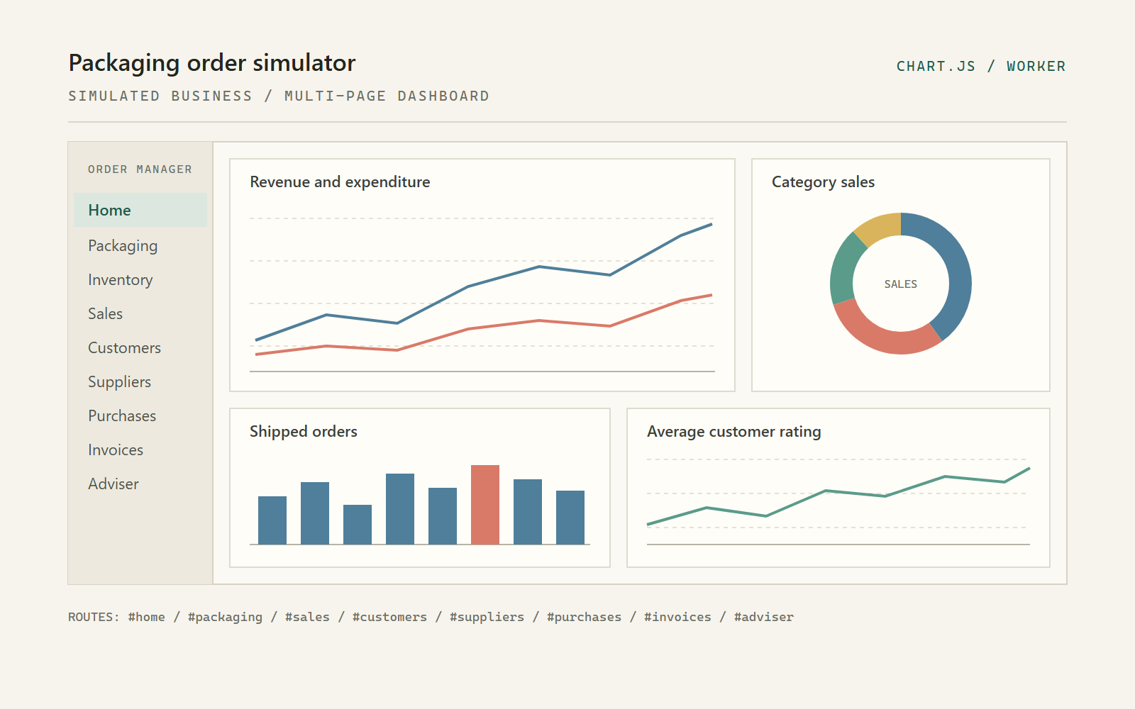
The packaging order simulator dashboard showing a revenue line chart, a category sales doughnut and two smaller charts.
Preview of the packaging order simulator demo.
06 Chart.js - 9 pages

Packaging order simulator

A simulated packaging business with nine pages, including sales, stock, customers and a procurement adviser. Orders are generated in a Web Worker, stored in IndexedDB and drawn with Chart.js.

Open demo

Six examples, each in its own folder.

Built with D3, Chart.js and Recharts.

01 - D3 v7 - SVG heatmap

Monthly temperature heatmap

The heatmap is built from a list of monthly temperature records. Each coloured square is an SVG <rect>, placed with D3 scales.

How it works

  1. Load the data. start() fetches a JSON file of { year, month, variance } records from the freeCodeCamp reference data. variance is the difference from the 1951-1980 average.
  2. Make three scales. Linear scales map year to x and month to y; a scaleQuantile maps variance to a 14-colour blue-to-red palette.
  3. Set up the chart area. The chart uses a margin convention: margins are subtracted from width and height, then a <g> is translated by the left and top margins. Axes are appended with axisBottom and axisLeft.
  4. Add the rectangles. selectAll('rect').data(...).enter().append('rect') creates one rectangle per month. x and y come from the scales; width and height are one cell. fill comes from the colour scale.
  5. Add a tooltip. On mouseover, d3.pointer() gives cursor coordinates inside the chart. The demo positions its custom <hoverTip> element there and writes the exact temperature, anomaly, month and year.
  6. Add a legend. A second data join creates the colour swatches below the chart.
const x = d3.scaleLinear().range([0, width - 50]);
const y = d3.scaleLinear().range([height - 100, 0]);
const colour = d3.scaleQuantile()
  .domain([buckets, lowTemp, d3.max(data, d => d.variance)])
  .range(colours);

chart.selectAll('.heat')
  .data(details.monthlyVariance)
  .enter()
  .append('rect')
  .attr('x', d => x(d.year))
  .attr('y', d => y(d.month))
  .attr('width', gridWidth)
  .attr('height', gridHeight)
  .style('fill', d => colour(d.variance));

Notes

  • scaleQuantile puts roughly the same number of values into each colour band. A linear colour scale would divide the value range evenly instead, which gives a different picture.
  • This example only passes a few values to the colour scale. A quantile scale normally gets every value, which spreads the colours out more evenly.
  • The chart has a fixed width, so it does not resize with the window. It still shows the usual margin setup.

Try it: change the colours array, or swap scaleQuantile for scaleLinear and compare the two versions.

Open the demo

02 - D3 v7 - TopoJSON - Choropleth

US education choropleth

The map uses two files: county boundaries in TopoJSON and education percentages in JSON. The two sets of data are matched by county FIPS code.

How it works

  1. Load the files. start() awaits the county boundaries and the education figures before drawing anything.
  2. Convert the map data. topojson.feature(topo, topo.objects.counties) expands shared borders into GeoJSON features, which makes the file smaller than one polygon per county.
  3. Draw the counties. d3.geoPath() converts each feature into SVG path data. These county coordinates are already projected, so no projection function is needed; with longitude and latitude you would pass something like d3.geoAlbersUsa().
  4. Choose the colours. d3.scaleThreshold() maps a percentage to one of eight green bands. A threshold scale gives clear colour bands, which are easier to show in a legend than a smooth gradient.
  5. Fill each county. One <path> is created per county. A lookup by FIPS finds the matching education record and drives fill.
  6. Add the legend. d3.legendColor() reads the scale, so the legend always matches the map.
const counties = topojson
  .feature(topo, topo.objects.counties)
  .features;

const colour = d3.scaleThreshold()
  .domain(d3.range(2.6, 75.1, (75.1 - 2.6) / 16))
  .range(d3.schemeGreens[8]);

svg.selectAll('path')
  .data(counties)
  .enter()
  .append('path')
  .attr('d', d3.geoPath())
  .attr('fill', d => {
    const county = education.find(e => e.fips === d.id);
    return county ? colour(county.bachelorsOrHigher) : '#ccc';
  });

Notes

  • Counties are matched by FIPS code, not name. County names repeat across states, but FIPS codes do not.
  • The code searches the education list for every county. That is fine for a demo, but a Map keyed by FIPS would be faster with larger data.
  • Counties with no matching record are left grey, so missing data is easy to spot.
  • A threshold scale hides the differences inside each colour band, but it makes the map easier to read.

Try it: swap schemeGreens for schemeBlues, or move one threshold and see how many counties change colour.

Open the demo

03 - D3 v7 - Hierarchy

Movie popularity treemap

A treemap shows the parts of a whole using area. The demo turns the movie data into a hierarchy, asks D3 to calculate a rectangle for each film, and draws them.

How it works

  1. Build the hierarchy. d3.hierarchy(data) creates parent and child nodes from the nested JSON.
  2. Add up the values. .sum(d => d.value) adds each movie's value up through its category, so parent rectangles know their total size.
  3. Calculate the layout. d3.treemap().size([1400, 550]).padding(1) runs the squarified algorithm and writes x0, y0, x1 and y1 onto every node.
  4. Draw the films. root.leaves() gives the movie nodes. Each gets a <g>, a <rect> sized from its corners, and a <foreignObject> so long titles can wrap inside the tile.
  5. Colour by category. scaleOrdinal maps the seven category names to fixed colours; a second group builds the legend from the same list.
  6. Add a tooltip. A tooltip shows the name, category and value, and stores the same values as data attributes.
const root = d3.treemap()
  .size([1400, 550])
  .padding(1)(
    d3.hierarchy(data)
      .sum(d => d.value)
      .sort((a, b) => a.value - b.value)
  );

root.leaves().forEach(movie => {
  // movie.x0, movie.y0, movie.x1, movie.y1
});

Notes

  • Area shows the value. Padding adds gaps between tiles but does not change their size.
  • Treemaps work well when there are many items. A pie chart with this many slices would be hard to read.
  • Small tiles cannot fit a label. This demo wraps text with foreignObject; many dashboards hide labels on small tiles and use a tooltip instead.
  • Sorting changes where the tiles go, not how big they are.

Try it: change padding(1) to paddingInner(3), or sort the other way and see where the tiles move.

Open the demo

04 - D3 v7 - Force simulation

Programming language influences

This is a force-directed graph, so there is no fixed layout. D3 treats the circles like charged particles and the links like springs, then redraws them on every tick.

How it works

  1. Read the data. Each language record has a linksTo array of names. The code converts those names into node indices to make { source, target } links.
  2. Size the circles. A circle's radius depends on how many other languages link to it, which gives a simple measure of influence.
  3. Start the simulation. d3.forceSimulation(nodes) combines forceLink (pull connected nodes together), forceManyBody (push everything apart), forceCollide (stop overlaps) and forceCenter (keep the graph on screen).
  4. Draw on every tick. The ticked handler creates or updates one <circle> per language and one <path> per link.
  5. Curve the lines. Each line is a quadratic curve: M source Q control target. The control point sits above the midpoint so the lines bow apart instead of overlapping.
  6. Add interaction. d3.drag() holds a circle in place with fx/fy while you drag it, and d3.zoom() moves the whole group. Clicking a circle fades the unrelated ones and opens a side panel.
const simulation = d3.forceSimulation(nodes)
  .force('link', d3.forceLink(links).distance(260))
  .force('charge', d3.forceManyBody())
  .force('collide', d3.forceCollide().radius(d => d.radius))
  .force('center', d3.forceCenter(width / 2, height / 2))
  .on('tick', ticked);

function ticked() {
  linkSelection.attr('d', d => curve(d));
  nodeSelection.attr('cx', d => d.x).attr('cy', d => d.y);
}

Notes

  • The simulation settles, but it is not fixed. Dragging a circle starts it moving again.
  • The links start as index numbers. Once the simulation runs, forceLink turns them into references to the circle objects.
  • Redrawing the SVG every tick is fine for a few dozen circles. With thousands, canvas or WebGL would be better.
  • Language names are cleaned up into valid IDs, so names with spaces or symbols still work.

Try it: increase distance(260), remove forceCollide, or add d3.forceRadial() to pull the circles into a ring.

Open the demo

05 - React - Recharts - Vite build

Salaries vs student loan thresholds

This is the only demo built with React. The chart is written as JSX, and Recharts handles the axes, scales and tooltips. Recharts uses D3 underneath.

How it works

  1. Store the data. An array holds one object per academic year: minimum wage, Plan 1 threshold, Plan 2 threshold, and a projected salary for the selected career.
  2. React updates the chart. Clicking a career button calls setCareer. React then redraws the salary line, cards and gap charts with the new value.
  3. Build the main chart. <ComposedChart> mixes four <Line> series. <ResponsiveContainer> sets the width. <XAxis>, <YAxis>, <CartesianGrid> and <Tooltip> draw the axes, grid and tooltip.
  4. Show the gap as bars. Two <BarChart>s plot salary minus threshold. A <ReferenceLine y={0}> marks the point where salary equals the threshold.
  5. Calculate repayments. Repayment is 9% of salary above the threshold; the cards divide that by 12 for a monthly figure.
  6. Leave gaps for missing years. Plan 2 did not exist before 2012, so its values are null and connectNulls={false} leaves a gap rather than inventing a line.
<ResponsiveContainer width="100%" height={500}>
  <ComposedChart data={historicalData}>
    <CartesianGrid strokeDasharray="3 3" />
    <XAxis dataKey="year" angle={-45} textAnchor="end" />
    <YAxis tickFormatter={formatCurrency} />
    <Tooltip content={<CustomTooltip />} />
    <Legend />
    <Line dataKey="minWageAnnual" name="Minimum Wage" />
    <Line dataKey="plan1Threshold" name="Plan 1 Threshold" />
    <Line dataKey="plan2Threshold" name="Plan 2 Threshold" connectNulls={false} />
    <Line dataKey="careerSalary" strokeDasharray="5 5" />
  </ComposedChart>
</ResponsiveContainer>

Notes

  • With Recharts you describe the chart instead of drawing the SVG yourself. That is a different way of working from the D3 examples.
  • The figures are not adjusted for inflation, and the salaries are estimates for entry-level roles. Treat it as an illustration, not financial advice.
  • Plan 1 and Plan 2 are different loan systems, so read the two gap charts separately.
  • The app is already built into the assets/ folder. The original JSX is not included, but you can read the compiled code in the bundle.

Try it: add another career to the configuration, or change the growth rate used to estimate past salaries.

Open the demo

06 - Chart.js 4 - Web Worker - IndexedDB

Packaging order simulator

This is a small application rather than a single chart. It simulates a packaging business and shows the results across nine pages, with tables, a dashboard, sales charts and a demand forecast.

How it works

  1. Start a worker. appWithWorker.js creates new Worker('sw.js'). Even though it is called sw.js, it is a Web Worker, not a service worker. It runs the simulation off the main thread so the page stays responsive.
  2. Generate and store. On first run, the worker creates customers, products, purchase orders, sales orders, invoices and daily counts, then writes them into IndexedDB (salesDB).
  3. Load a page. The URL hash (#home, #sales, #packaging and so on) is sent to the worker as a message. messageHandler.js reads the matching data store and rebuilds the page; DataTables adds sorting and search to the tables.
  4. Draw the charts. Chart.js draws onto <canvas>. The dashboard has a pie chart and a set of smaller line and bar charts. The sales page has a daily, weekly or monthly line chart.
  5. Replace old charts. Before a new Chart.js instance is created, the old one is destroyed. Otherwise canvases and event listeners pile up.
  6. Forecast demand. The adviser module runs a Bayesian-style update per week and product, then plots forecast mean, uncertainty and actual demand on one chart.
// charts.js - one line chart, rebuilt on each period change
if (chart) chart.destroy();

chart = new Chart(document.getElementById('myChart'), {
  type: 'line',
  data: {
    labels: data.labels,
    datasets: [{
      label: `Value of ${period} Sales`,
      data: data.values,
      borderWidth: 1,
      tension: 0.3
    }]
  },
  options: { responsive: true }
});

Notes

  • Chart.js draws on a canvas, while the D3 demos create SVG elements. Canvas is faster with lots of points, but you cannot style or inspect individual bars with CSS.
  • The pages are controlled by the URL hash. Changing the hash sends a new request to the worker, so each page is the same document with different content.
  • Everything runs in the browser, with no server. Regenerating deletes and recreates the IndexedDB database, so it takes a moment.
  • The forecast chart changes the line style when data is missing or falling. That is a simple way to show uncertainty.

Try it: open the menu and change the date range or starting budget, then regenerate. Compare the new dashboard with the old one.

Open the demo